¦ HOME ¦ Math Software Downloads ¦ Numerical Methods ¦ Register Your Software ¦ Contact ¦ Search ¦ Credit ¦

Software:
Linear Algebra
Functions
Ordinary Differential Equations
Systems of Nonlinear Equations
Multiple Integration
Maxima and Minima
Functions and Equations
Regression
Approximation & Interpolation
Stereographer
Math Miscellanea
Support Software
Numerical Methods:
Integration and Differentiation
Solution of Equations
Maxima and Minima
Approximation of Functions
Regression
Polynomial Regression
Fast Fourier Transforms
Differential Equations
Linear Algebra Methods
Miscellaneous Procedures
Decimal Comma/Decimal Point                             

Enter your search terms Submit search form   Web www.numericalmathematics.com

	Upon registering, you will receive by email a liberation key which will remove the registration reminder and the time limitation. You will be entitled to one year of free updates.

Click here to download FUNCTIONS Requirements: Windows 98 or later

AWARDS

Click here to download FUNCTIONS Requirements: Windows 98 or later

The first thing to do is to provide the function to be studied. For this go to the area next to "f(x)=":

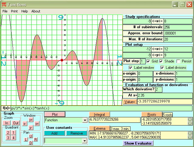
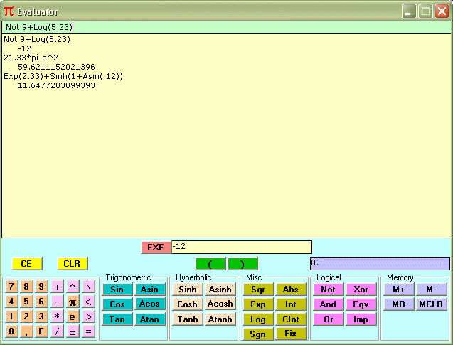
f(x)= Enter the function in terms of “x” and the user constants you define. See Available Functions, Operators and Constants for details on what is available.

If you wish to define any constants, do this under User constants. Type the definition (For instance, age=32.5) and click Add or press Enter. To remove a constant, select it from the list and click Remove. A constant can be defined by an expression, for instance rec=sin(1)/exp(3.44).

Now we should specify the details for the study of the function. Go to the area Study specifications:

(Interval lower limit) <= x <= (Interval upper limit)

Enter the lower and upper limits of the interval.

# of subintervals: This is the number of subintervals you wish to use. A plot of the function will give a very good idea of how many intervals you should specify keeping the following in mind:

When searching for roots and maxima and minima, too few subintervals may result in missing some good candidates for a solution because they are first detected by changes in signs in a subinterval so only one would be found per subinterval. On the other hand, specifying too many may result in a very time-consuming search.

When performing integration, the number of subintervals is really the MINIMUM number of subintervals because an adaptable integration scheme is used and these will be adjusted until the error bound is met.

Approx. error bound: Maximum error you wish in the calculations.

The program uses algorithms that generate successive approximations sequences. It starts by assuming that a value is close to a solution. Suppose this value is x₀. Using an algorithm the program finds a closer approximation to the solution. Suppose this is x₁. We may now use x₁ as an initial approximation and apply the algorithm to obtain an even closer approximation x₂. This process is continued until the current approximation in the sequence differs from the previous approximation by less than the specified error.

Max. # of iterations: If a particular attempt is not converging, the main iteration loop would be executed endlessly. This provides an escape by limiting the number of iterations.

Now you're ready to obtain some results.

Click on Integral to compute the integral of the function over the interval specified. If necessary do the integration piecewise, each time selecting an interval in which the function is continuous and well-behaved.

Click on Extrema to find the maxima and minima of the function in the given interval. The output shows whether it is a maximum or a minimum, the x value at which it occurs and the value of the function at that point. For example,

MAX: [x1,y1]
MIN: [x2,y2]

Click on Roots to find the function's roots in the given interval. The x values at which the roots occur will be displayed.

To find any derivative of the function at any given x, go to Evaluation of function or derivatives and enter the order of the derivative (0 for the function itself, 1 for the first derivative, 2 for the second, etc.) and the point at which you want it evaluated. Click Value to compute the value.

First and second derivatives will generally be fairly accurate. Higher order derivatives are computed using a general formula and the error will usually be greater as the order increases. If you need higher accuracy, especially with derivatives of order 3 or higher, a better idea may be to approximate the function by a power or trigonometric series using a program of the APPROXIMATION & INTERPOLATION set, then use the results with the POWER AND TRIGONOMETRIC SERIES program. If you know the general term which generates the coefficients of a Taylor or Fourier series expansion of the function, then you can use the GENERATE program to find a finite (truncated) series approximation.

To set up a plot go to Plot setup. Here you to set the position of the relative axes, define the window, select the plotting step, specify the distance between the divisions on the axes, decide if you want a grid on the graph and whether or not you want the graphics to be persistent. The details follow.

Define the window for plotting by entering the ranges of the variables:

(x lower limit) <= x <= (x upper limit)
(y lower limit) <= y <= (y upper limit)

If you think of the plotting region as a window, this will allow you to place it anywhere in the x-y plane and give you a view as wide or as narrow as you wish in both directions.

To enter the plotting step go to

Plot step:

This must be an integer between 1 and 80, and determines the points at which the function or derivative is evaluated when plotting. A step of 1 gives the sharpest plot and requires evaluation at every horizontal pixel position. Other choices are faster. For example, a step of 10 only requires evaluation every 10 positions.

Choose the relative origin of the axes you want on the plot:

x-origin:
y-origin:

You can set them anywhere, although usually you would want them at (0,0).

Set the divisions you wish to put on each of the axes:

x-divisions:
y-divisions:

These divisions will be placed starting from the (relative) origin.

If you want a grid on the graph, place a checkmark next to Grid. Instead of divisions on the axes, a grid will be plotted.

If you place a checkmark on Shade, the area between the function and the (relative) x-axis will be shaded.

Placing a checkmark on Label window will place labels on the edges of the window.

Putting a checkmark on Label divisions will label the divisions you place on the axes.

By placing a checkmark next to Persist the graphics drawn will be persistent, meaning they will be automatically redrawn if they hide behind another window and later re-appear.

Under the button named Plot there is a drop-down list of options:

Function
1st. Derivative
2nd. Derivative
3rd. Derivative
4th. Derivative
5th. Derivative
6th. Derivative
7th. Derivative
8th. Derivative
9th. Derivative

Select one of the options to plot the solution or any one of its first nine derivatives.

Click on Plot to display a graph of the selected option.

Under Graph you can manipulate the displayed graph:

Zoom in or out by clicking on In or Out.

Click on 1, 2, 3 or 4 to magnify the corresponding quadrant.

Click on L, U, R or D to pan left, up, right or down.

Click x+, x-, y+ or y- to make the window wider or narrower in the x or y direction.

If you click on the graph the plot will be centered on the point you click.

On the top bar, the File option let’s you save the function and any results to disk, or retrieve a previously created file. You can also copy the graph to the clipboard, which you can then paste where you please (Word, Paint, etc.).

NOTE: The graph will also be saved using the name you specify but with the .BMP extension (BITMAP).

Use the Print option to print the results.

Click on SHOW EVALUATOR to display the expression evaluator.

Available Functions

Available Operators

The operators are listed below in order of precedence.

Comparison Operators (These all have EQUAL precedence)

Built-in Constants

The constants pi and e are built-in for your convenience:

pi = 3.14159… = atn(1)*4

e = 2.718281… = exp(1)

Copyright © 2001-2010 Numerical Mathematics. All rights reserved.